COUNTIF and IFERROR – Excel Formula with example

How efficient are you in Excel? Do you take too long on Excel tasks and feel frustrated that you are doing one thing over and over?  Excel is one of the most efficient programs if you know how to apply Excel formulas to your tasks. You will be surprised at how powerful Excel can get when fed with the right formulas. Excel formulas are very useful in handling large data sets efficiently. The good thing is that these formulas are very easy to learn. To understand this better, it is good to practice on excel formula with example.

Top Excel Functions with Formula examples (Tutorial 1: COUNTIF & IFERROR)

ماذا is COUNTIF FUNCTION

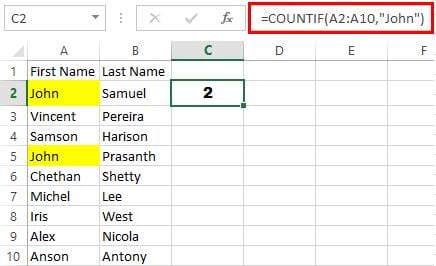
The COUNTIF function is used to show how many times a certain value appears. The formula is written as;

How to use COUNTIF Function:

=COUNTIF (range, criteria)

If for example, you have a list of 50 names and would like to see how many times the name John appears in column A, the formula would be;

=COUNTIF (A2: A50, “John”)

Pin

If this formula were to be used for other columns, it would have to be manually changed every time for a new column. To avoid this, absolute references are made. This would be written as;

=COUNTIF ($A$2:$A$50, “$D11”) where D11 is the new cell it has been copied into.

Click here to read more on COUNTIF excel formula with example screenshots! (Count cells between two numbers using COUNIF formula)

ماذا is IFERROR Function

Though this function is not a common appearance in the list of Excel formulas, it is very useful in handling errors.  This function is used to avoid error messages. When Excel encounters an error, it will often show up as #VALUE!.  Other error messages that come up include are #DIV.  The IFERROR function is written as;

How to use IFERROR Function:

=IFERROR (condition/value, what result if condition/value is wrong).

If for example there is a division formula in C2 that is A2/B2, the IFERROR formula would be written as; =IFERROR (A2/b2, “Review”) to avoid an error message. The word ‘Review’ would show up when Excel encounters a difficulty in executing the division formula if for example there is a text value that cannot be divided.

Screenshot example and scenarios (to make it more simple to understand):

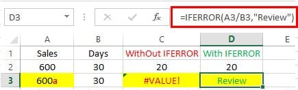
Scenario 1. Direct division formula without IFERROR function

600/30 = 20 {Formula in C2 =A2/B2}

Scenario 2. Direct division formula without IFERROR function where value contains a text

600a/30 = #VALUE! {Formula in C3 =A3/B3}

Scenario 3. Division formula with IFERROR function

600/30 =20 {Formula in D2 =IFERROR (A2/B2,”Review”)}

Scenario 4. Division formula with IFERROR function where value contains a text.

600a/30 =مراجعة {Formula in D3 =IFERROR (A2/B2,”Review”)}